Feature Engineering for AI

Feature Engineering

• การบวนการใช้ความรู้ Domain Knowledge ในการสร้าง Feature ใหม่ขึ้นมา ตัด Feature ที่ไม่เกี่ยวข้องทิ้งไป เพื่อช่วยทำให้อัลกอริทึมเรียนรู้ได้ดีขึ้น

เทคนิคในการทำ Feature Engineering มีทั้งหมด 7 วิธี ได้แก่

• 1. Imputation
• 2. Handling Outliers
• 3. Drop Outlier with Standard Deviation
• 4. Drop with Percentiles
• 5. Binning
• 6. Log Transform
• 7. One-Hot Encoding

ในขั้นตอนแรกสิ่ที่สำคัญที่สุด คือ >> Understanding Data Quality

• คือ การสำรวจข้อมูลเพื่อพิจารณาคุณภาพในแง่ต่างๆ แล้วจึงเลือกเทคนิคในการทำ Feature Engineering ที่เหมาะสมและต้องมีการนำเข้า library ของ pandas ก่อนเพื่อเข้าใจคุณลักษณะของข้อมูลได้อย่างรวดเร็ว โดยคำนวณมาจากค่าสถิติต่างๆ ด้วย ProfileReport Function และoutput ที่เข้าใจง่าย
• ติดตั้ง Pandas Profiling Library ด้วยคำสั่ง pip install

pip install pandas-profiling[notebook]

• เตรียม Dataset และเรียกใช้ ProfileReport Function บน Jupyter Notebook

import numpy as np
import pandas as pd
from pandas_profiling import ProfileReport

• Load dataset จาก “titanic.csv” แล้วเรียกข้อมูลทั้งหมด

df = pd.read_csv("titanic.csv")
df

• ต่อไปเรียกใช้ ProfileReport Function เพื่อรายงานผลข้อมูล

profile = ProfileReport(df, title="Pandas Profiling Report")
profile

• ใช้ isnull() และ sum() ในการหาค่า Missing Values

print(df.isnull().sum())

ต่อไปจะเข้าสู่ขั้นตอนการทำ Feature Engineering

1. Imputation

• คือการแทนที่ค่าที่หายไป ด้วยค่าค่าหนึ่ง ด้วยฟังก์ชัน fillna()

new_df = df.copy()
new_df[‘Age’].fillna(df[‘Age’].mean(), inplace = True)print(new_df.isnull().sum())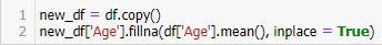

• และหาค่า Missing Values ใหม่ โดยใช้ isnull() และ sum()

print(new_df.isnull().sum())

• จะเห็นว่าค่าของ Age จะเป็น 0
• จากการกำหนดค่า Threshold ดังตัวอย่างด้านล่าง จะทำให้ Column ที่มีร้อยละของ Missing Value มากกว่า 50% คือ Column Cabin ถูกลบ

df.isnull().mean()

threshold = 0.5
new_df = df[df.columns[df.isnull().mean() < threshold]]new_df.isnull().mean()

• และหาค่า mean ใหม่ จะได้

new_df.isnull().mean()

• ขณะที่การลบ Row ที่มีร้อยละของ Missing Value มากกว่า 50% จะใช้คำสั่ง

print(df.shape)
new_df = df.loc[df.isnull().mean(axis=1) < threshold]
print(new_df.shape)

print(new_df.isnull().sum())

2. Handling Outliers

• เป็นวิธีที่ใช้จัดการกับ ค่าที่มีค่าออกมาโดดๆ เป็นส่วนที่เรียกว่า Outliner

import seaborn as sns
from matplotlib import pyplot as plt

plt.show()fig = plt.figure(figsize=(12,8))
sns.boxplot(x=df['Age'], color='red')
plt.xlabel('Age Featured', fontsize=14)
plt.show()

df['Age'].describe()

3. Drop Outlier with Standard Deviation

print(df.shape)
factor = 3
upper_lim = df['Age'].mean () + df['Age'].std () * factor
lower_lim = df['Age'].mean () - df['Age'].std () * factor
drop_outlier1 = df[(df['Age'] < upper_lim) & (df['Age'] > lower_lim)]
print(drop_outlier1.shape)

fig = plt.figure(figsize=(12,8))
sns.boxplot(x=drop_outlier1['Age'], color='red')
plt.xlabel('Age Featured', fontsize=14)
plt.show()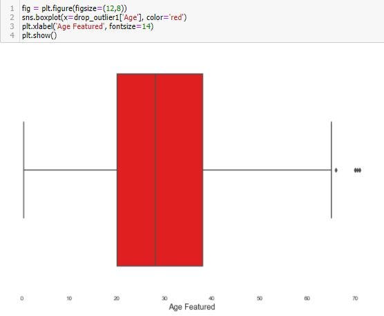

drop_outlier1['Age'].describe()

4. Drop with Percentiles

• นอกจากนี้เราสามารถลบแถวที่พบ Outlier ใน Column price ที่น้อยกว่าหรือเท่ากับ Quantile 0.5 และมากกว่าหรือเท่ากับ Quantile 0.95

print(df.shape)
upper_lim = df['Age'].quantile(.95)
lower_lim = df['Age'].quantile(.05)
drop_outlier2 = df[(df['Age'] < upper_lim) & (df['Age'] > lower_lim)]
print(drop_outlier2.shape)

fig = plt.figure(figsize=(12,8))
sns.boxplot(x=drop_outlier2['Age'], color='red')
plt.xlabel('Age Featured', fontsize=14)
plt.show()

drop_outlier2['Age'].describe()

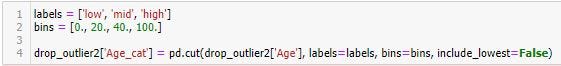
5. Binning

• จัดกลุ่มให้กับข้อมูล การทำ Binning หรือการแบ่งข้อมูลออกตามช่วงที่กำหนด จะทำให้สามารถป้องกันการเกิด Overfitting เมื่อมีการ Train Model ได้ในระดับหนึ่ง
• เช่น การแบ่งราคาไวน์เป็น Low, Mid, High ตามช่วง bin = [0, 20, 40, 100]

labels = ['low', 'mid', 'high']
bins = [0., 20., 40., 100.]
drop_outlier2['Age_cat'] = pd.cut(drop_outlier2['Age'], labels=labels, bins=bins, include_lowest=False)

drop_outlier2.sample(n=5).head(5)

6. Log Transform

• Log Transform เป็นการใช้ Log ทางคณิตศาสตร์แปลงข้อมูล ซึ่งจะช่วยลดการเบ้ของข้อมูล โดยหลังการแปลงข้อมูลแล้ว จะทำให้การกระจายตัวเข้าสู่ Normal Distribution มากขึ้น

drop_outlier2['log'] = (drop_outlier2['Age']).transform(np.log)

drop_outlier2.sample(n=5).head()

7. One-hot encoding

• One-hot Encoding เป็นการเข้ารหัสข้อมูลแบบหนึ่งที่มักจะใช้กันบ่อยในงานทางด้าน Machine Learning โดยการขยายข้อมูลจากเดิมที่มี Column เดียว เป็นค่า 0 และ 1 หลายๆ Column ตามจำนวนหมวดหมู่ของข้อมูลใน Column เดิม โดยจะมีการกำหนดค่าเป็น 1 ใน Column ใหม่ และตำแหล่งของ Column จะแทนลำดับของหมวดหมู่ของข้อมูลเดิม แล้วกำหนดค่า 0 ใน Column อื่นๆ ที่เหลือ

encoded_columns = pd.get_dummies(drop_outlier2['Age_cat'])
drop_outlier2 = drop_outlier2.join(encoded_columns)

drop_outlier2.sample(n=5).head()

สำหรับวันนี้ก็ขอจบการใช้ Feature Engineering เพียงเท่านี้

<<ขอบคุณครับ>>