Implement the Back-propagation Algorithm with Numpy

Phakorn
6 min readAug 25, 2020

<< Perceptron >>

  • Perceptron (P) เป็น Neural Network อย่างง่าย ที่จำลองการทำงานของเซลล์ประสาทมนุษย์ โดยประกอบด้วย Input layers หรือเรียกอีกอย่างหนึ่งว่า Input Node มีทั้งหมด 2 cell และ Output layer เรียกอีกอย่างหนึ่งว่า Output Node มีทั้งหมด 1 cell

Forward Propagation

Input Layer

  • จากภาพด้านบน Node ที่มีสีฟ้า คือ Input Data (Xi) ที่จะเป็นข้อมูลแบบ Scalar, Vector หรือ Matrix
Xi, i ∈ 1, 2

Output Layer

  • ส่วน Layer สุดท้ายของ Neural Network คือ Output Layer ที่เป็น Node สีส้ม และ Node สีนำ้ตาล โดยที่ Node สีส้ม จะมีการนำ Weight ที่เกิดจากการสุ่มในช่วงเริ่มต้นของการ Train คูณกับ Input Data แล้วนำผลลัพธ์จากการคูณมาบวกกับ Bias (B) ซึ่งเกิดจากการสุ่มในช่วงเริ่มต้นเช่นกัน
Z = W · X + B
  • ในการ Implement เราจะแทน Weight (W) ด้วย Matrix ขนาด mxn โดย m คือจำนวน Output Node (ในที่นี้มี 1 Node) และ n คือ จำนวน Input Node (ในที่นี้มี 2 Node)
W = [w1 w2]
  • และ B เป็น Matrix ขนาด mx1
B = [b]
  • ดังนั้น Z จะเท่ากับ 0.36
Z = [w1x1 + w2x2] + [b]
= [(0.2)(0.05) + (0.5)(0.1)] + [0.3]
= [0.36]

Activate Function

  • จะทำให้ค่านอยู่ในช่วง 0–1 ซึ่งเราเรียกฟังก์ชันสำหรับการปรับค่าอย่างนี้ว่า Activate Function
  • ดังนั้นผลลัพธ์สุดท้ายที่เป็นค่าที่ Model ทำนายออกมาได้ หรือ ŷ จะเท่ากับ Sigmoid(z)
ŷ = Sigmoid(z) = Sigmoid(0.36) = 0.5890

Loss Function

  • ขั้นตอนสุดท้ายของการทำ Forward Propagation คือการประเมินว่าผลการ Predict คลาดเคลื่อนจาก Output y มากน้อยเพียงใด
L = Loss(y,ŷ) 
= (y - ŷ)^2
= (0.7 - 0.589)^2 = 0.0123

Back-propagation

>> Implement with NumPy <<

  • เราจะทดลอง Implement Neural Network โดยเพิ่มความซับซ้อนของ Model อีกเล็กน้อย ดังภาพด้านล่าง
  • เราสามารถทำกระบวนการ Backward Propagation เพื่อปรับค่า w1 จากการหาอนุพันธ์ของ L เทียบกับ w1 หรือความชัน (Gradient) ของ Loss(y, ŷ) หรือ Error ที่ w1 ลองเปลี่ยนเป็นW2จะได้ดังภาพ
  • ค่าที่ได้ Error_at_w2 = (-0.222)(0.242)(0.1) = -0.005
  • ต่อมาให้เราปรับ Learning Rate เท่ากับ 0.5 เพื่อนำมาปรับค่า w2
Update w2 = w2 — Learning_Rate*Error_at_w2
= 0.5-(0.5)(-0.005)
= 0.5025

นิยาม Neural Network Model ที่ไม่ใส่ Bias

class NeuralNetwork:
def __init__(self, x, y):
self.input = x
self.weights1 = np.random.rand(self.input.shape[1],4)
self.weights2 = np.random.rand(4,1)
self.y = y
self.output = np.zeros(y.shape)
  • กำหนดค่า X และ y
import numpy as np

X = np.array([[0,0,1],
[0,1,1],
[1,0,1],
[1,1,1]])

y = np.array([[0],[1],[1],[0]])
X.shape, y.shape

สร้าง nn1 แล้ว Print ค่าต่างๆ

nn1 = NeuralNetwork(X,y)nn1.input.shape
print(nn1.input)
nn1.weights1.shape
print(nn1.weights1)
nn1.weights2.shape
print(nn1.weights2)
nn1.y.shape
print(nn1.y)
nn1.output.shape
print(nn1.output)

นิยาม Neural Network Class

  • ในขั้นตอนนี้เราจะทำการหาค่า learning_rate ตั้งแต่ 0.1 > 1.0 จึงต้องใส่ loss ตัวอื่นเพิ่มเข้าไป ดังตัวอย่างด้านล่าง
import numpy as np

def sigmoid(x):
return 1.0/(1+ np.exp(-x))

def sigmoid_derivative(x):
return x * (1.0 - x)

class NeuralNetwork:
def __init__(self, x, y, l):
self.input = x
self.weights1 = np.random.rand(self.input.shape[1],4)
self.weights2 = np.random.rand(4,1)
self.y = y
self.output = np.zeros(self.y.shape)
self.learning_rate = l

def loss(self):
return sum((self.y - self.output)**2)
def loss2(self):
return sum((self.y - self.output)**2)
def loss3(self):
return sum((self.y - self.output)**2)
def loss4(self):
return sum((self.y - self.output)**2)
def loss5(self):
return sum((self.y - self.output)**2)
def loss6(self):
return sum((self.y - self.output)**2)
def loss7(self):
return sum((self.y - self.output)**2)
def loss8(self):
return sum((self.y - self.output)**2)
def loss9(self):
return sum((self.y - self.output)**2)
def loss10(self):
return sum((self.y - self.output)**2)
def feedforward(self):
self.layer1 = sigmoid(np.dot(self.input, self.weights1))
self.output = sigmoid(np.dot(self.layer1, self.weights2))

def backprop(self):
d_weights2 = np.dot(self.layer1.T, (2*(self.y - self.output) * sigmoid_derivative(self.output)))
d_weights1 = np.dot(self.input.T, (np.dot(2*(self.y - self.output) * sigmoid_derivative(self.output), self.weights2.T) * sigmoid_derivative(self.layer1)))

self.weights1 += self.learning_rate*d_weights1
self.weights2 += self.learning_rate*d_weights2

Train Model

  • จะ Train Model ของ learning_rate ตั้งแต่ 0.1 > 1.0 ดังตัวอย่างด้านล่าง
learning_rate = 0.1
nn = NeuralNetwork(X,y,learning_rate)
loss=[]
for i in range(1000):
nn.feedforward()
nn.backprop()
loss.append(nn.loss())

learning_rate = 0.2
nn2 = NeuralNetwork(X,y,learning_rate)
loss2=[]
for i in range(1000):
nn2.feedforward()
nn2.backprop()
loss2.append(nn2.loss2())

learning_rate = 0.3
nn3 = NeuralNetwork(X,y,learning_rate)
loss3=[]
for i in range(1000):
nn3.feedforward()
nn3.backprop()
loss3.append(nn3.loss())

learning_rate = 0.4
nn4 = NeuralNetwork(X,y,learning_rate)
loss4=[]
for i in range(1000):
nn4.feedforward()
nn4.backprop()
loss4.append(nn4.loss4())

learning_rate = 0.5
nn5 = NeuralNetwork(X,y,learning_rate)
loss5=[]
for i in range(1000):
nn5.feedforward()
nn5.backprop()
loss5.append(nn5.loss5())

learning_rate = 0.6
nn6 = NeuralNetwork(X,y,learning_rate)
loss6=[]
for i in range(1000):
nn6.feedforward()
nn6.backprop()
loss6.append(nn6.loss6())

learning_rate = 0.7
nn7 = NeuralNetwork(X,y,learning_rate)
loss7=[]
for i in range(1000):
nn7.feedforward()
nn7.backprop()
loss7.append(nn7.loss7())

learning_rate = 0.8
nn8 = NeuralNetwork(X,y,learning_rate)
loss8=[]
for i in range(1000):
nn8.feedforward()
nn8.backprop()
loss8.append(nn8.loss8())

learning_rate = 0.9
nn9 = NeuralNetwork(X,y,learning_rate)
loss9=[]
for i in range(1000):
nn9.feedforward()
nn9.backprop()
loss9.append(nn9.loss9())

learning_rate = 1.0
nn10 = NeuralNetwork(X,y,learning_rate)
loss10=[]
for i in range(1000):
nn10.feedforward()
nn10.backprop()
loss10.append(nn10.loss10())

Plot Loss

import pandas as pd
from matplotlib import pyplot as plt
%matplotlib inline
df = pd.DataFrame(loss, columns=['loss'])
df1 = pd.DataFrame(loss2, columns=['loss2'])
df2 = pd.DataFrame(loss3, columns=['loss3'])
df3 = pd.DataFrame(loss4, columns=['loss4'])
df4 = pd.DataFrame(loss5, columns=['loss5'])
df5 = pd.DataFrame(loss6, columns=['loss6'])
df6 = pd.DataFrame(loss7, columns=['loss7'])
df7 = pd.DataFrame(loss8, columns=['loss8'])
df8 = pd.DataFrame(loss9, columns=['loss9'])
df9 = pd.DataFrame(loss10, columns=['loss10'])
import plotly
import plotly.graph_objs as go
plotly.offline.init_notebook_mode(connected=True)

h1 = go.Scatter(y=df['loss'],
mode="lines", line=dict(
width=2,
color='blue'),
name="loss")

h2 = go.Scatter(y=df1['loss2'],
mode="lines", line=dict(
width=2,
color='red'),
name="0.2")
h3 = go.Scatter(y=df2['loss3'],
mode="lines", line=dict(
width=2,
color='lightgrey'),
name="0.3")
h4 = go.Scatter(y=df3['loss4'],
mode="lines", line=dict(
width=2,
color='pink'),
name="0.4")
h5 = go.Scatter(y=df4['loss5'],
mode="lines", line=dict(
width=2,
color='grey'),
name="0.5")
h6 = go.Scatter(y=df5['loss6'],
mode="lines", line=dict(
width=2,
color='orange'),
name="0.6")
h7 = go.Scatter(y=df6['loss7'],
mode="lines", line=dict(
width=2,
color='black'),
name="0.7")
h8 = go.Scatter(y=df7['loss8'],
mode="lines", line=dict(
width=2,
color='violet'),
name="0.8")
h9 = go.Scatter(y=df8['loss9'],
mode="lines", line=dict(
width=2,
color='yellow'),
name="0.9")
h10 = go.Scatter(y=df9['loss10'],
mode="lines", line=dict(
width=2,
color='rosybrown'),
name="1.0")
data = [h1, h2, h3, h4, h5, h6, h7, h8, h9, h10]

layout1 = go.Layout(title='Loss',
xaxis=dict(title='epochs'),
yaxis=dict(title=''))
fig1 = go.Figure(data, layout=layout1)
plotly.offline.iplot(fig1)
  • กราฟจะได้ ดังนี้

วิเคราะห์ผลการทดลอง

  • วิเคราะห์ผลจากกราฟที่ทำการเปลี่ยนค่า learning_rate ไปเรื่อยๆตั้งแต่ 0.1–1.0 และให้ทำการเปลี่ยน h1 ไปเรื่อยๆจนถึง h10 จะเห็นได้ว่าค่า learning_rate มีผลกับค่า loss ยิ่งค่าของ learning_rate มากขึ้นจะทำให้ค่า loss น้อยลงดังตัวอย่างข้างต้น

Sign up to discover human stories that deepen your understanding of the world.

No responses yet

Write a response